[1]:

import pyAMARES

pyAMARES.__version__

[1]:

'0.3.21'

Examples of In Vivo X-Nuclei (\(^{129}\)Xe and \(^{2}\)H) MRS Fitting

Reproduce Figures 2B, C and Figures S2C, D of the pyAMARES publication

Try this tutorial on Google Colab!

Fitting a Voxel of Hyperpolarized \(^{129}\)Xe MRSI Acquired from Healthy Porcine Lungs at 3T

Set Scanner Parameters:
- MHz (Field Strength): 35.340772 MHz, corresponding to \(^{129}\)Xe at 3T
- sw (Spectral Width): 20000 Hz
- Deadtime: 7.14e-05 seconds

[2]:

MHz = 35.340772
sw = 20000
begin_time = 7.14e-05

Load the FID of an Example Voxel of \(^{129}\)Xe MRSI

[3]:

fid = pyAMARES.readmrs("attachment/a_voxel_Xe.txt")

Try to load 2-column ASCII data
data.shape= (256,)

Initialize the FID Object

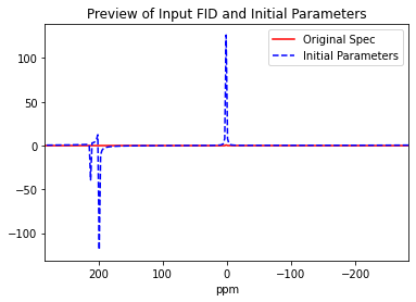
[4]:

# Initialize an FIDobj using the loaded fid and spectral parameters
FIDobj = pyAMARES.initialize_FID(
    fid,
    priorknowledgefile="attachment/FigS2A.csv",  # Prior knowledge file for hyperpolarized 129Xe
    MHz=MHz,
    sw=sw,
    deadtime=begin_time,
    preview=True,
    g_global=False,
)  # When g_global is False, the lineshape parameter `g` will be fitted based on prior knowledge constraints

Checking comment lines in the prior knowledge file
Parameter g will be fit with the initial value set in the file attachment/FigS2A.csv

../_images/notebooks_X-Nuclei_Example_8_1.png

Printing the Prior Knowledge File attachment/FigS2A.csv

	Gas	Membrane	RBC
Index
Initial Values	NaN	NaN	NaN
amplitude	1	0.6	0.2
chemicalshift	0	197	210
linewidth	40	10	10
phase	0	0	Membrane
g	0	0.1	0
Bounds	NaN	NaN	NaN
amplitude	(0,	(0,	(0,
chemicalshift	(-25,25)	(192, 205)	(200,215)
linewidth	(0,	(0,200)	(0,200)
phase	(-180,180)	(-180,180)	(-180,180)
g	(0,1)	(0,1)	(0,1)

Note: In the prior knowledge dataset, the gas and red blood cell (RBC) signals are modeled with Lorentzian lineshapes (g = 0), while the membrane signal is modeled with a Voigt lineshape (initial value: g = 0.1) to account for its structural heterogeneity. This approach has become widely accepted in the xenon MRS community for quantifying membrane and RBC signals Bier et al., NMR Biomed. 2019

First Round of Fitting: Parameter Optimization

[5]:

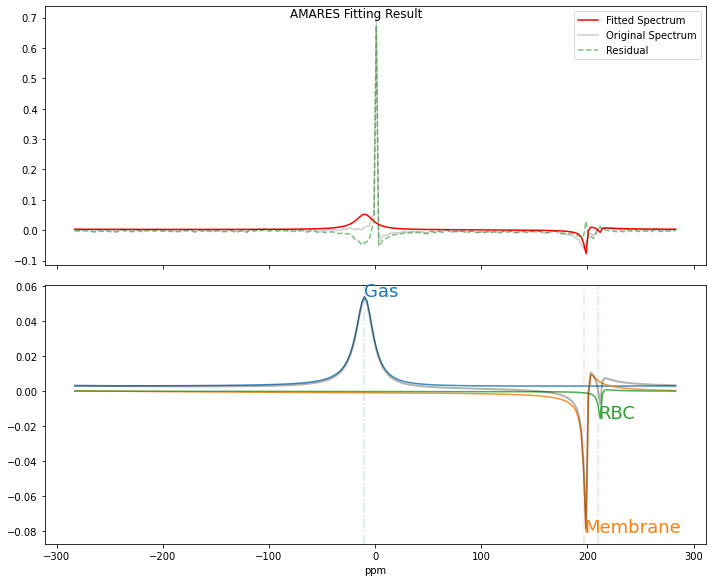
out1 = pyAMARES.fitAMARES(
    fid_parameters=FIDobj,
    fitting_parameters=FIDobj.initialParams,
    method="leastsq",  # Initialize parameters using the Levenberg-Marquardt method
    ifplot=True,
    inplace=False,
)

A copy of the input fid_parameters will be returned because inplace=False
Autogenerated tol is 7.601e-08
Fitting with method=leastsq took 0.231262 seconds
Estimated CRLBs are calculated using the default noise variance estimation used by OXSA.
a_sd is all None, use crlb instead!
freq_sd is all None, use crlb instead!
lw_sd is all None, use crlb instead!
phase_sd is all None, use crlb instead!
g_std is all None, use crlb instead!
It seems that zeros are padded after 85
Remove padded zeros from residual estimation!
Lmfit Fitting Results:
----------------
Number of function evaluations (nfev): 1000
Reduced chi-squared (redchi): 6.892370384435103e-06
Fit success status: Failure
Fit message: Tolerance seems to be too small. Could not estimate error-bars.
Norm of residual = 0.003
Norm of the data = 0.000
resNormSq / dataNormSq = 23.631

/home/jxu125/git/pyamares/pyAMARES/util/crlb.py:54: RuntimeWarning: Warning: The matrix may be ill-conditioned. Condition number is high: 1.965e+19
  warnings.warn(

../_images/notebooks_X-Nuclei_Example_11_2.png

Optimized Fitting Parameters

[6]:

out1.fittedParams

[6]:

name	value	initial value	min	max	vary	expression
ak_Gas	0.00652552	1.0	0.00000000	inf	True
freq_Gas	-379.033205	0.0	-883.519300	883.519300	True
dk_Gas	2182.09753	125.66370614359172	0.00000000	inf	True
phi_Gas	0.11411036	0.0	-3.14159265	3.14159265	True
g_Gas	5.6341e-09	0.0	0.00000000	1.00000000	True
ak_Membrane	0.00164767	0.6	0.00000000	inf	True
freq_Membrane	6965.79679	6962.132084	6785.42822	7244.85826	True
dk_Membrane	351.070545	31.41592653589793	0.00000000	628.318531	True
phi_Membrane	-0.65148111	0.0	-3.14159265	3.14159265	True
g_Membrane	5.7732e-15	0.1	0.00000000	1.00000000	True
ak_RBC	2.7290e-04	0.2	0.00000000	inf	True
freq_RBC	7427.30605	7421.5621200000005	7068.15440	7598.26598	True
dk_RBC	327.926634	31.41592653589793	0.00000000	628.318531	True
phi_RBC	-0.65148111	0.0	-3.14159265	3.14159265	False	phi_Membrane
g_RBC	0.02854482	0.0	0.00000000	1.00000000	True

Fix Lineshape Parameters of Gas and RBC for the AMARES Fitting

[7]:

out1.fittedParams["g_Gas"].vary = False
out1.fittedParams["g_RBC"].vary = False

[8]:

out1.fittedParams

[8]:

name	value	initial value	min	max	vary	expression
ak_Gas	0.00652552	1.0	0.00000000	inf	True
freq_Gas	-379.033205	0.0	-883.519300	883.519300	True
dk_Gas	2182.09753	125.66370614359172	0.00000000	inf	True
phi_Gas	0.11411036	0.0	-3.14159265	3.14159265	True
g_Gas	5.6341e-09	0.0	0.00000000	1.00000000	False
ak_Membrane	0.00164767	0.6	0.00000000	inf	True
freq_Membrane	6965.79679	6962.132084	6785.42822	7244.85826	True
dk_Membrane	351.070545	31.41592653589793	0.00000000	628.318531	True
phi_Membrane	-0.65148111	0.0	-3.14159265	3.14159265	True
g_Membrane	5.7732e-15	0.1	0.00000000	1.00000000	True
ak_RBC	2.7290e-04	0.2	0.00000000	inf	True
freq_RBC	7427.30605	7421.5621200000005	7068.15440	7598.26598	True
dk_RBC	327.926634	31.41592653589793	0.00000000	628.318531	True
phi_RBC	-0.65148111	0.0	-3.14159265	3.14159265	False	phi_Membrane
g_RBC	0.02854482	0.0	0.00000000	1.00000000	False

Fitting AMARES Using Levenberg-Marquardt-Initialized Parameters:

[9]:

out2 = pyAMARES.fitAMARES(
    fid_parameters=out1,
    fitting_parameters=out1.fittedParams,  # Fit Xenon data using optimized parameters with fixed g_Gas and g_RBC
    method="least_squares",
    ifplot=True,
    inplace=False,
)

A copy of the input fid_parameters will be returned because inplace=False
Autogenerated tol is 7.601e-08
Fitting with method=least_squares took 0.125702 seconds
Estimated CRLBs are calculated using the default noise variance estimation used by OXSA.
It seems that zeros are padded after 85
Remove padded zeros from residual estimation!
Lmfit Fitting Results:
----------------
Number of function evaluations (nfev): 46
Reduced chi-squared (redchi): 3.930007675969261e-08
Fit success status: Success
Fit message: `gtol` termination condition is satisfied.
Norm of residual = 0.000
Norm of the data = 0.000
resNormSq / dataNormSq = 0.135

/home/jxu125/git/pyamares/pyAMARES/util/crlb.py:54: RuntimeWarning: Warning: The matrix may be ill-conditioned. Condition number is high: 2.980e+18
  warnings.warn(

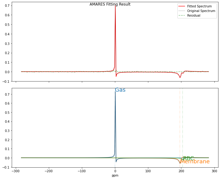
../_images/notebooks_X-Nuclei_Example_18_2.png

Visualization of AMARES Fitting as shown in Figure 2B of pyAMARES Publication

[10]:

# Modify the visualization parameters
plotParameters = out2.plotParameters
plotParameters.xlim = (300, -300)  # Show spectrum from 300 to -300 ppm
plotParameters.ifphase = False  # Do not apply phase correction
plotParameters.lb = 5  # Apply line broadening of 5 Hz for visualization

[11]:

pyAMARES.plotAMARES(out2, plotParameters=plotParameters)

fitting_parameters is None, just use the fid_parameters.out_obj.params

../_images/notebooks_X-Nuclei_Example_21_1.png

Obtained Fitting Results Spreadsheet as shown in Figure S2C of pyAMARES Publication

[12]:

out2.simple_df

[12]:

	amplitude	chem shift(ppm)	LW(Hz)	phase(deg)	SNR	CRLB(%)
name
Gas	0.004	0.062	6.106	-44.828	10.185	0.487
Membrane	0.002	196.127	200.000	-39.198	5.355	4.745
RBC	0.001	204.617	200.000	-39.198	2.156	12.295

Fitting a Voxel of \(^{2}\)H 3D MRSI Acquired at 3T

Set Scanner Parameters:
- MHz (Field Strength): 19.613053 MHz, corresponding to \(^{2}\)H at 3T
- sw (Spectral Width): 5000 Hz
- Deadtime: 0 seconds

[13]:

MHz = 19.613053
sw = 5000
begin_time = 0

Load the FID of an Example Voxel of \(^{2}\)H 3D MRSI

[14]:

fid = pyAMARES.readmrs("attachment/a_voxel_2HMRSI.txt")
fid.shape

Try to load 2-column ASCII data
data.shape= (1400,)

[14]:

(1400,)

Initialize the FID Object

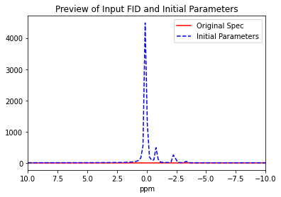
[15]:

FIDobj = pyAMARES.initialize_FID(
    fid,
    priorknowledgefile="attachment/FigS2B.csv",  # Prior knowledge file for 2H 3D MRSI analysis
    MHz=MHz,
    sw=sw,
    deadtime=begin_time,
    preview=True,
    xlim=(10, -10),  # Spectral visualization range: -10 to 10 ppm
    ppm_offset=-4.7,  # Adjust DHO peak to 0 ppm by setting ppm_offset to -4.7 ppm
    g_global=0.8,  # Set Voigt lineshape g=0.8
)

Checking comment lines in the prior knowledge file
Shifting the ppm by ppm_offset=-4.70 ppm
before opts.initialParams[freq_DHO].value=92.1813491
new value should be opts.initialParams[freq_DHO].value + opts.ppm_offset * opts.MHz=0.0
after opts.initialParams[freq_DHO].value=0.0
before opts.initialParams[freq_Glucose].value=74.5296014
new value should be opts.initialParams[freq_Glucose].value + opts.ppm_offset * opts.MHz=-17.6517477
after opts.initialParams[freq_Glucose].value=-17.6517477
before opts.initialParams[freq_Glx].value=45.1100219
new value should be opts.initialParams[freq_Glx].value + opts.ppm_offset * opts.MHz=-47.071327200000006
after opts.initialParams[freq_Glx].value=-47.071327200000006
before opts.initialParams[freq_Lactate].value=25.496968900000002
new value should be opts.initialParams[freq_Lactate].value + opts.ppm_offset * opts.MHz=-66.6843802
after opts.initialParams[freq_Lactate].value=-66.6843802

../_images/notebooks_X-Nuclei_Example_29_1.png

Printing the Prior Knowledge File attachment/FigS2B.csv

	DHO	Glucose	Glx	Lactate
Index
Initial Values	NaN	NaN	NaN	NaN
amplitude	10	1	0.7	0.1
chemicalshift	4.7	3.8	2.3	1.3
linewidth	10	10	10	10
phase	0	DHO	DHO	DHO
g	0	0	0	0
Bounds	NaN	NaN	NaN	NaN
amplitude	(0,	(0,	(0,	(0,
chemicalshift	(4.2, 5.2)	(3.3, 4.3)	(1.8,2.8)	(0.8, 1.8)
linewidth	(0,	(0,100)	(0,100)	(0, 100)
phase	(-180,180)	(-180,180)	(-180,180)	(-180,180)
g	(0,1)	(0,1)	(0,1)	(0,1)

AMARES Fitting with an Internal Levenberg-Marquardt Parameter Initializer

[16]:

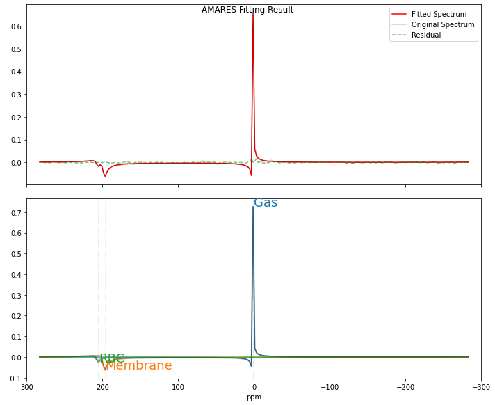
out1 = pyAMARES.fitAMARES(
    fid_parameters=FIDobj,
    fitting_parameters=FIDobj.initialParams,
    method="least_squares",
    ifplot=True,
    inplace=False,
    initialize_with_lm=True,
)  # Levenberg-Marquardt initializer is executed internally

A copy of the input fid_parameters will be returned because inplace=False
Autogenerated tol is 1.109e-07
Run internal leastsq initializer to optimize fitting parameters for the next least_squares fitting
Fitting with method=leastsq took 0.600929 seconds
Fitting with method=least_squares took 0.270947 seconds
Estimated CRLBs are calculated using the default noise variance estimation used by OXSA.
It seems that zeros are padded after 700
Remove padded zeros from residual estimation!
Lmfit Fitting Results:
----------------
Number of function evaluations (nfev): 5
Reduced chi-squared (redchi): 9.417199596703771e-07
Fit success status: Success
Fit message: `ftol` termination condition is satisfied.
Norm of residual = 0.003
Norm of the data = 0.005
resNormSq / dataNormSq = 0.569

/home/jxu125/git/pyamares/pyAMARES/util/crlb.py:54: RuntimeWarning: Warning: The matrix may be ill-conditioned. Condition number is high: 4.480e+12
  warnings.warn(

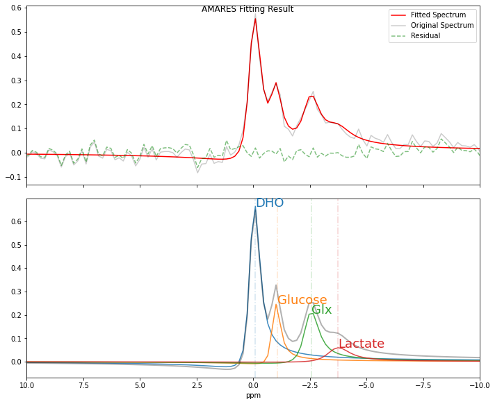
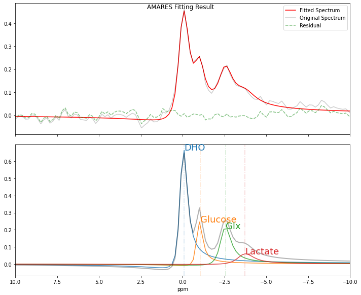
../_images/notebooks_X-Nuclei_Example_31_2.png

Visualization of AMARES Fitting as shown in Figure 2D of pyAMARES Publication

[24]:

# Modify the visualization parameters
plotParameters = out1.plotParameters
plotParameters.ifphase = False  # Do not apply phase correction
plotParameters.lb = 5.0  # Apply line broadening of 5 Hz for visualization
plotParameters.xlim = (10, -10)  # Show spectrum from 10 to -10 ppm

[25]:

pyAMARES.plotAMARES(fid_parameters=out1, plotParameters=plotParameters)

fitting_parameters is None, just use the fid_parameters.out_obj.params

../_images/notebooks_X-Nuclei_Example_34_1.png

Obtained Fitting Results Spreadsheet as shown in Figure S2D of pyAMARES Publication

[26]:

out1.simple_df

[26]:

	amplitude	chem shift(ppm)	LW(Hz)	phase(deg)	SNR	CRLB(%)
name
DHO	0.004	-0.090	39.679	-19.241	2.361	4.619
Glucose	0.001	-1.052	30.113	-19.241	0.682	13.969
Glx	0.002	-2.571	60.789	-19.241	1.088	19.562
Lactate	0.001	-3.733	100.000	-19.241	0.476	54.700

[ ]: