[1]:
import pyAMARES
import numpy as np

pyAMARES.__version__
[1]:
'0.3.15'
Fitting Simulated In Vivo 31P MRS Data
Try This Tutorial on Google Colab!
Simulating an In Vivo MRS Spectrum
Load Prior Knowledge: Use the dataset based on the 7T brain data reported by Ren et al. in NMR Biomedicine, 28(11): 1455–1462.
[2]:
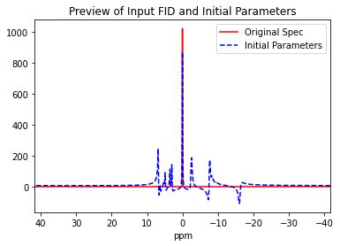
priorknowledge = pyAMARES.initialize_FID(
    fid=None,
    priorknowledgefile="./attachment/example_human_brain_31P_7T_flex_phase.csv",
    preview=True,
)
Warning, fid is None!
Checking comment lines in the prior knowledge file
Comment: in line 0 "#  Ren et al, NMR Biomed . 2015 Nov;28(11):1455-62. doi: 10.1002/nbm.3384.",,,,,,,,,,,,,,,,

Comment: in line 14 # Phase not fixed ,,,,,,,,,,,,,,,,

Comment: in line 15 " # 2024/06/24 In Ren et al, the chemical shift range of BATP (0.1 ppm), AATP (0.04 ppm), and GATP (0.02 ppm) are smaller than the J-couplin range (0.125 - 0.25 ppm). ",,,,,,,,,,,,,,,,

Comment: in line 16 "# So, increase the chemical shift range",,,,,,,,,,,,,,,,
Printing the Prior Knowledge File ./attachment/example_human_brain_31P_7T_flex_phase.csv
| BATP | BATP2 | BATP3 | AATP | AATP2 | GATP | GATP2 | UDPG | NAD | PCr | GPC | GPE | Pin | Pex | PC | PE | |
|---|---|---|---|---|---|---|---|---|---|---|---|---|---|---|---|---|
| Index | ||||||||||||||||
| Initial Values | NaN | NaN | NaN | NaN | NaN | NaN | NaN | NaN | NaN | NaN | NaN | NaN | NaN | NaN | NaN | NaN |
| amplitude | 1.41 | BATP/2 | BATP/2 | 1.545 | AATP | 1.5 | GATP | 0.08 | 0.41 | 4.37 | 1.32 | 0.8 | 0.85 | 0.3 | 0.3 | 2.27 |
| chemicalshift | -16.15 | BATP-15Hz | BATP+15Hz | -7.49 | AATP-16Hz | -2.46 | GATP-16Hz | -9.72 | -8.25 | 0 | 2.95 | 3.5 | 4.82 | 5.24 | 6.24 | 6.76 |
| linewidth | 58.12 | BATP | BATP | 32.28 | AATP | 39.02 | GATP | 32.37 | 40.49 | 15.41 | 19.96 | 19.1 | 21.04 | 30.91 | 19.96 | 22.63 |
| phase | 0 | BATP | BATP | 0 | AATP | 0 | GATP | 0 | 0 | 0 | 0 | 0 | 0 | 0 | 0 | 0 |
| g | 0 | 0 | 0 | 0 | 0 | 0 | 0 | 0 | 0 | 0 | 0 | 0 | 0 | 0 | 0 | 0 |
| Bounds | NaN | NaN | NaN | NaN | NaN | NaN | NaN | NaN | NaN | NaN | NaN | NaN | NaN | NaN | NaN | NaN |
| amplitude | (0, | (0, | (0, | (0, | (0, | (0, | (0, | (0, | (0, | (0, | (0, | (0, | (0, | (0, | (0, | (0, |
| chemicalshift | (-16.30,-16.00) | (-16.30,-16.00) | (-16.30,-16.00) | (-7.72,-7.42) | (-7.72,-7.42) | (-2.65,-2.39) | (-2.65,-2.39) | (-9.76,-9.68) | (-8.25,-8.17) | (-0.5, 0.5) | (2.94,2.96) | (3.49,3.51) | (4.81,4.83) | (5.19,5.29) | (6.22,6.26) | (6.71,6.81) |
| linewidth | (54.335, 61.911) | (54.335, 61.911) | (54.335, 61.911) | (31.226, 33.327) | (31.226, 33.327) | (36.892, 41.157) | (36.892, 41.157) | (29.125, 35.619) | (34.823, 46.155) | (13.21, 17.603) | (18.557, 21.359) | (17.348, 20.849) | (19.353, 22.727) | (22.091, 39.725) | (15.756, 24.16) | (20.658, 24.605) |
| phase | (-180, 180) | (-180, 180) | (-180, 180) | (-180, 180) | (-180, 180) | (-180, 180) | (-180, 180) | (-180, 180) | (-180, 180) | (-180, 180) | (-180, 180) | (-180, 180) | (-180, 180) | (-180, 180) | (-180, 180) | (-180, 180) |
| g | (0,1) | (0,1) | (0,1) | (0,1) | (0,1) | (0,1) | (0,1) | (0,1) | (0,1) | (0,1) | (0,1) | (0,1) | (0,1) | (0,1) | (0,1) | (0,1) |
| # 2024/06/24 In Ren et al, the chemical shift range of BATP (0.1 ppm), AATP (0.04 ppm), and GATP (0.02 ppm) are smaller than the J-couplin range (0.125 - 0.25 ppm). | NaN | NaN | NaN | NaN | NaN | NaN | NaN | NaN | NaN | NaN | NaN | NaN | NaN | NaN | NaN | NaN |
| # So, increase the chemical shift range | NaN | NaN | NaN | NaN | NaN | NaN | NaN | NaN | NaN | NaN | NaN | NaN | NaN | NaN | NaN | NaN |
| NaN | NaN | NaN | NaN | NaN | NaN | NaN | NaN | NaN | NaN | NaN | NaN | NaN | NaN | NaN | NaN | NaN |
Perturb Peak Parameters: Randomly adjust the 31P spectra peak parameters by 5%, chemical shift by 10 Hz
[3]:
from copy import deepcopy
[4]:
params0 = deepcopy(
    priorknowledge.initialParams
)  # Make a copy of initialParams to be perturbed
[5]:
def perturb_value(value, percentage=5):
    percentage = float(percentage)
    # Generate a random perturbation factor between 0.95 and 1.05
    factor = np.random.uniform(1 - percentage / 100, 1 + percentage / 100)
    # Apply the perturbation factor
    result = value * factor
    # print(f"Perturbing input {value=} to {result=}")
    return result


def perturb_table(inputparams, percentage=5, freq_shift=5, phase_shift=0):
    params = deepcopy(inputparams)
    for i in params:
        if params[i].name.startswith("ak") or params[i].name.startswith("dk"):
            params[i].value = perturb_value(params[i].value)
        if params[i].name.startswith("freq"):
            params[i].value += np.random.uniform(-freq_shift, freq_shift)
        if params[i].name.startswith("phi"):
            params[i].value += np.random.uniform(
                -np.deg2rad(phase_shift), np.deg2rad(phase_shift)
            )
    return params
[6]:
params = perturb_table(params0, percentage=5, freq_shift=5, phase_shift=0)
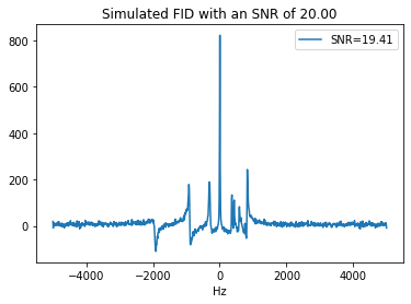
Simulate the 31P MRS Spectra Using Scanner Parameters:
MHz (Field Strength): 120 MHz, corresponding to 31P at 7T.
sw (Spectral Width): 10000.0 Hz.
Deadtime: 200 microseconds (200e-6 seconds).
Number of Points (fid_len): 1024.
SNR (Signal to Noise Ratio, snr_target): 20.
[7]:
fid = pyAMARES.kernel.fid.simulate_fid(
    params,
    MHz=120.0,
    sw=10000.0,
    deadtime=200e-6,
    fid_len=1024,
    snr_target=20,
    preview=True,
)
Simple Tutorial on pyAMARES Fitting
Initialize the FID Object:
[8]:
FIDobj = pyAMARES.initialize_FID(
    fid=fid,
    MHz=120.0,
    sw=10000.0,
    deadtime=200e-6,
    normalize_fid=False,
    priorknowledgefile="./attachment/example_human_brain_31P_7T_flex_phase.csv",
    preview=False,
)
Checking comment lines in the prior knowledge file
Comment: in line 0 "#  Ren et al, NMR Biomed . 2015 Nov;28(11):1455-62. doi: 10.1002/nbm.3384.",,,,,,,,,,,,,,,,

Comment: in line 14 # Phase not fixed ,,,,,,,,,,,,,,,,

Comment: in line 15 " # 2024/06/24 In Ren et al, the chemical shift range of BATP (0.1 ppm), AATP (0.04 ppm), and GATP (0.02 ppm) are smaller than the J-couplin range (0.125 - 0.25 ppm). ",,,,,,,,,,,,,,,,

Comment: in line 16 "# So, increase the chemical shift range",,,,,,,,,,,,,,,,
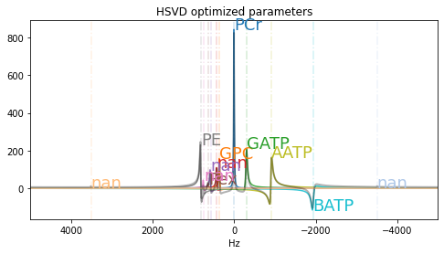
A. HSVD Optimization of Initial Parameters (Optional): Utilize HSVD to optimize the initial parameters for fitting, if desired.
[9]:
params_hsvd = pyAMARES.HSVDinitializer(
    fid_parameters=FIDobj,
    num_of_component=12,  # If error happens, decreasae this number
    fitting_parameters=FIDobj.initialParams,
    preview=True,
)
Norm of residual = 65.858
Norm of the data = 2408.147
resNormSq / dataNormSq = 0.027
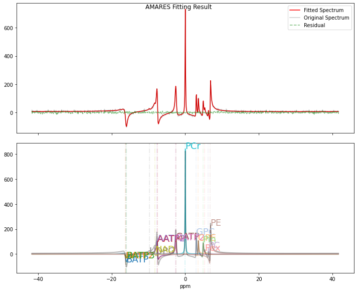
Fitting AMARES Using HSVD-Initialized Parameters:
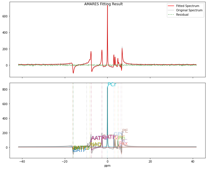
[10]:
FIDresult1 = pyAMARES.fitAMARES(
    fid_parameters=FIDobj,
    fitting_parameters=params_hsvd,
    method="least_squares",
    ifplot=True,
    inplace=False,
)
A copy of the input fid_parameters will be returned because inplace=False
Autogenerated tol is 3.158e-06
Fitting with method=least_squares took 5.937595 seconds
Estimated CRLBs are calculated using the default noise variance estimation used by OXSA.
Lmfit Fitting Results:
----------------
Number of function evaluations (nfev): 15
Reduced chi-squared (redchi): 0.030735869137296347
Fit success status: Success
Fit message: `ftol` termination condition is satisfied.
Norm of residual = 61.472
Norm of the data = 2408.147
resNormSq / dataNormSq = 0.026
[11]:
FIDresult1.styled_df
[11]:
| amplitude | sd | CRLB(%) | chem shift(ppm) | sd(ppm) | CRLB(cs%) | LW(Hz) | sd(Hz) | CRLB(LW%) | phase(deg) | sd(deg) | CRLB(phase%) | g | g_sd | g (%) | SNR | |
|---|---|---|---|---|---|---|---|---|---|---|---|---|---|---|---|---|
| name | ||||||||||||||||
| BATP | 2.774 | 0.056 | 2.795 | -16.123 | 0.010 | 0.068 | 61.099 | 1.958 | 4.287 | -1.814 | 1.113 | 88.258 | 0.000 | 0.000 | nan | 11.133 |
| AATP | 3.037 | 0.068 | 3.121 | -7.512 | 0.004 | 0.077 | 31.613 | 0.996 | 4.376 | -0.015 | 1.288 | 11728.739 | 0.000 | 0.000 | nan | 12.187 |
| GATP | 2.914 | 0.044 | 2.112 | -2.484 | 0.004 | 0.211 | 36.104 | 0.906 | 3.483 | -0.368 | 0.871 | 328.653 | 0.000 | 0.000 | nan | 11.694 |
| UDPG | 0.071 | 0.038 | 73.621 | -9.760 | 0.080 | 1.142 | 27.638 | 19.262 | 96.796 | 44.761 | 30.378 | 94.238 | 0.000 | 0.000 | nan | 0.286 |
| NAD | 0.441 | 0.078 | 24.589 | -8.250 | 0.036 | 0.609 | 46.155 | 8.687 | 26.131 | -3.662 | 10.139 | 384.739 | 0.000 | 0.000 | nan | 1.771 |
| PCr | 4.159 | 0.025 | 0.842 | -0.012 | 0.001 | 6.211 | 15.005 | 0.126 | 1.166 | -0.142 | 0.347 | 340.441 | 0.000 | 0.000 | nan | 16.692 |
| GPC | 1.208 | 0.033 | 3.848 | 2.953 | 0.003 | 0.130 | 18.826 | 0.663 | 4.893 | -1.532 | 1.588 | 143.921 | 0.000 | 0.000 | nan | 4.848 |
| GPE | 0.873 | 0.035 | 5.500 | 3.510 | 0.004 | 0.156 | 19.040 | 0.947 | 6.904 | 2.568 | 2.269 | 122.719 | 0.000 | 0.000 | nan | 3.503 |
| Pin | 0.909 | 0.045 | 6.935 | 4.810 | 0.005 | 0.157 | 22.727 | 1.307 | 7.987 | 2.573 | 2.862 | 154.417 | 0.000 | 0.000 | nan | 3.646 |
| Pex | 0.219 | 0.043 | 27.094 | 5.242 | 0.019 | 0.495 | 20.041 | 4.489 | 31.101 | -0.272 | 11.179 | 5697.685 | 0.000 | 0.000 | nan | 0.881 |
| PC | 0.332 | 0.035 | 14.789 | 6.220 | 0.010 | 0.224 | 18.355 | 2.404 | 18.188 | -8.989 | 6.102 | 94.260 | 0.000 | 0.000 | nan | 1.334 |
| PE | 2.281 | 0.039 | 2.348 | 6.790 | 0.002 | 0.042 | 23.277 | 0.492 | 2.935 | 0.706 | 0.969 | 190.518 | 0.000 | 0.000 | nan | 9.155 |
B. Initialization Using Levenberg-Marquardt Method: Instead of using the HSVD initializer, initialize the parameters using the Levenberg-Marquardt method.
[12]:
params_LM = pyAMARES.fitAMARES(
    fid_parameters=FIDobj,
    fitting_parameters=FIDobj.initialParams,
    method="leastsq",
    ifplot=True,
    inplace=False,
)
A copy of the input fid_parameters will be returned because inplace=False
Autogenerated tol is 3.158e-06
Fitting with method=leastsq took 3.309779 seconds
Estimated CRLBs are calculated using the default noise variance estimation used by OXSA.
a_sd is all None, use crlb instead!
freq_sd is all None, use crlb instead!
lw_sd is all None, use crlb instead!
phase_sd is all None, use crlb instead!
g_std is all None, use crlb instead!
Lmfit Fitting Results:
----------------
Number of function evaluations (nfev): 595
Reduced chi-squared (redchi): 0.034074975457039455
Fit success status: Success
Fit message: Fit succeeded. Could not estimate error-bars.
Norm of residual = 68.150
Norm of the data = 2408.147
resNormSq / dataNormSq = 0.028
Fitting AMARES Using Levenberg-Marquardt-Initialized Parameters:
[13]:
FIDresult2 = pyAMARES.fitAMARES(
    fid_parameters=FIDobj,
    fitting_parameters=params_LM.fittedParams,
    initialize_with_lm=False,
    method="least_squares",
    ifplot=True,
    inplace=False,
)
A copy of the input fid_parameters will be returned because inplace=False
Autogenerated tol is 3.158e-06
Fitting with method=least_squares took 2.848357 seconds
Estimated CRLBs are calculated using the default noise variance estimation used by OXSA.
Lmfit Fitting Results:
----------------
Number of function evaluations (nfev): 7
Reduced chi-squared (redchi): 0.030735869852873087
Fit success status: Success
Fit message: `ftol` termination condition is satisfied.
Norm of residual = 61.472
Norm of the data = 2408.147
resNormSq / dataNormSq = 0.026

[14]:
FIDresult2.styled_df
[14]:
| amplitude | sd | CRLB(%) | chem shift(ppm) | sd(ppm) | CRLB(cs%) | LW(Hz) | sd(Hz) | CRLB(LW%) | phase(deg) | sd(deg) | CRLB(phase%) | g | g_sd | g (%) | SNR | |
|---|---|---|---|---|---|---|---|---|---|---|---|---|---|---|---|---|
| name | ||||||||||||||||
| BATP | 2.774 | 0.056 | 2.795 | -16.123 | 0.010 | 0.068 | 61.099 | 1.958 | 4.287 | -1.814 | 1.113 | 88.257 | 0.000 | 0.000 | nan | 11.133 |
| AATP | 3.037 | 0.068 | 3.121 | -7.512 | 0.004 | 0.077 | 31.614 | 0.996 | 4.376 | -0.015 | 1.288 | 11709.060 | 0.000 | 0.000 | nan | 12.187 |
| GATP | 2.914 | 0.044 | 2.112 | -2.484 | 0.004 | 0.211 | 36.104 | 0.906 | 3.483 | -0.368 | 0.871 | 328.587 | 0.000 | 0.000 | nan | 11.694 |
| UDPG | 0.071 | 0.038 | 73.624 | -9.760 | 0.080 | 1.142 | 27.634 | 19.260 | 96.801 | 44.759 | 30.380 | 94.246 | 0.000 | 0.000 | nan | 0.286 |
| NAD | 0.441 | 0.078 | 24.589 | -8.250 | 0.036 | 0.609 | 46.155 | 8.687 | 26.130 | -3.662 | 10.139 | 384.695 | 0.000 | 0.000 | nan | 1.771 |
| PCr | 4.159 | 0.025 | 0.842 | -0.012 | 0.001 | 6.211 | 15.005 | 0.126 | 1.166 | -0.142 | 0.347 | 340.405 | 0.000 | 0.000 | nan | 16.692 |
| GPC | 1.208 | 0.033 | 3.848 | 2.953 | 0.003 | 0.130 | 18.826 | 0.663 | 4.893 | -1.532 | 1.588 | 143.915 | 0.000 | 0.000 | nan | 4.848 |
| GPE | 0.873 | 0.035 | 5.500 | 3.510 | 0.004 | 0.156 | 19.040 | 0.947 | 6.904 | 2.568 | 2.269 | 122.723 | 0.000 | 0.000 | nan | 3.503 |
| Pin | 0.909 | 0.045 | 6.935 | 4.810 | 0.005 | 0.157 | 22.727 | 1.307 | 7.987 | 2.573 | 2.862 | 154.405 | 0.000 | 0.000 | nan | 3.646 |
| Pex | 0.219 | 0.043 | 27.093 | 5.242 | 0.019 | 0.495 | 20.041 | 4.489 | 31.101 | -0.281 | 11.179 | 5530.322 | 0.000 | 0.000 | nan | 0.881 |
| PC | 0.332 | 0.035 | 14.789 | 6.220 | 0.010 | 0.224 | 18.356 | 2.404 | 18.187 | -8.991 | 6.102 | 94.245 | 0.000 | 0.000 | nan | 1.334 |
| PE | 2.281 | 0.039 | 2.348 | 6.790 | 0.002 | 0.042 | 23.277 | 0.492 | 2.935 | 0.707 | 0.969 | 190.440 | 0.000 | 0.000 | nan | 9.155 |
New after 0.3.10: Fitting AMARES using internally initialized Levenberg-Marquardt parameters:
[15]:
FIDresult2b = pyAMARES.fitAMARES(
    fid_parameters=FIDobj,
    fitting_parameters=FIDobj.initialParams,
    initialize_with_lm=True,  # Turn on the Levenberg-Marquardt initializer
    method="least_squares",
    ifplot=True,
    inplace=False,
)
A copy of the input fid_parameters will be returned because inplace=False
Autogenerated tol is 3.158e-06
Run internal leastsq initializer to optimize fitting parameters for the next least_squares fitting
Fitting with method=leastsq took 3.33159 seconds
Fitting with method=least_squares took 3.026501 seconds
Estimated CRLBs are calculated using the default noise variance estimation used by OXSA.
Lmfit Fitting Results:
----------------
Number of function evaluations (nfev): 7
Reduced chi-squared (redchi): 0.030735869852873087
Fit success status: Success
Fit message: `ftol` termination condition is satisfied.
Norm of residual = 61.472
Norm of the data = 2408.147
resNormSq / dataNormSq = 0.026

[16]:
FIDresult2b.styled_df
[16]:
| amplitude | sd | CRLB(%) | chem shift(ppm) | sd(ppm) | CRLB(cs%) | LW(Hz) | sd(Hz) | CRLB(LW%) | phase(deg) | sd(deg) | CRLB(phase%) | g | g_sd | g (%) | SNR | |
|---|---|---|---|---|---|---|---|---|---|---|---|---|---|---|---|---|
| name | ||||||||||||||||
| BATP | 2.774 | 0.056 | 2.795 | -16.123 | 0.010 | 0.068 | 61.099 | 1.958 | 4.287 | -1.814 | 1.113 | 88.257 | 0.000 | 0.000 | nan | 11.133 |
| AATP | 3.037 | 0.068 | 3.121 | -7.512 | 0.004 | 0.077 | 31.614 | 0.996 | 4.376 | -0.015 | 1.288 | 11709.060 | 0.000 | 0.000 | nan | 12.187 |
| GATP | 2.914 | 0.044 | 2.112 | -2.484 | 0.004 | 0.211 | 36.104 | 0.906 | 3.483 | -0.368 | 0.871 | 328.587 | 0.000 | 0.000 | nan | 11.694 |
| UDPG | 0.071 | 0.038 | 73.624 | -9.760 | 0.080 | 1.142 | 27.634 | 19.260 | 96.801 | 44.759 | 30.380 | 94.246 | 0.000 | 0.000 | nan | 0.286 |
| NAD | 0.441 | 0.078 | 24.589 | -8.250 | 0.036 | 0.609 | 46.155 | 8.687 | 26.130 | -3.662 | 10.139 | 384.695 | 0.000 | 0.000 | nan | 1.771 |
| PCr | 4.159 | 0.025 | 0.842 | -0.012 | 0.001 | 6.211 | 15.005 | 0.126 | 1.166 | -0.142 | 0.347 | 340.405 | 0.000 | 0.000 | nan | 16.692 |
| GPC | 1.208 | 0.033 | 3.848 | 2.953 | 0.003 | 0.130 | 18.826 | 0.663 | 4.893 | -1.532 | 1.588 | 143.915 | 0.000 | 0.000 | nan | 4.848 |
| GPE | 0.873 | 0.035 | 5.500 | 3.510 | 0.004 | 0.156 | 19.040 | 0.947 | 6.904 | 2.568 | 2.269 | 122.723 | 0.000 | 0.000 | nan | 3.503 |
| Pin | 0.909 | 0.045 | 6.935 | 4.810 | 0.005 | 0.157 | 22.727 | 1.307 | 7.987 | 2.573 | 2.862 | 154.405 | 0.000 | 0.000 | nan | 3.646 |
| Pex | 0.219 | 0.043 | 27.093 | 5.242 | 0.019 | 0.495 | 20.041 | 4.489 | 31.101 | -0.281 | 11.179 | 5530.322 | 0.000 | 0.000 | nan | 0.881 |
| PC | 0.332 | 0.035 | 14.789 | 6.220 | 0.010 | 0.224 | 18.356 | 2.404 | 18.187 | -8.991 | 6.102 | 94.245 | 0.000 | 0.000 | nan | 1.334 |
| PE | 2.281 | 0.039 | 2.348 | 6.790 | 0.002 | 0.042 | 23.277 | 0.492 | 2.935 | 0.707 | 0.969 | 190.440 | 0.000 | 0.000 | nan | 9.155 |
Visualize Fitting Results
Visualization with pyAMARES: pyAMARES utilizes the
plotParameterobject to display fitting results visually.Template for ``plotParameter``: Within the initialized
FIDobj, there is a pre-configured template forplotParameterto facilitate customization and usage.
[17]:
plotParameter = (
    FIDobj.plotParameters
)  # plotParameter is a pointer to FIDobj.plotParameters
# If you do not want to modify FIDobj.plotParameters,
# do plotParameter = deepcopy(FIDobj.plotParameters) instead
plotParameter
[17]:
Namespace(deadtime=0.0002, ifphase=False, lb=2.0, sw=10000.0, xlim=None)
Modify the visualization parameters
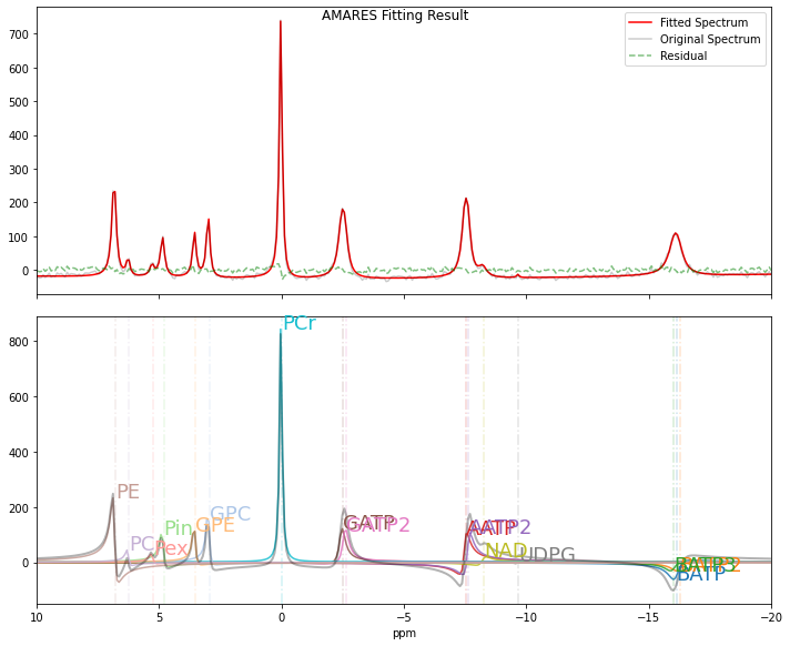
[18]:
plotParameter.ifphase = True  # Phasing the spectrum for visualization
plotParameter.xlim = (10, -20)  # Show 10 to -20 ppm only
[19]:
pyAMARES.plotAMARES(FIDresult2, plotParameters=plotParameter)
fitting_parameters is None, just use the fid_parameters.out_obj.params

Uniform Phase for All Peaks: Previously, each peak’s phase was fitted independently. We can now attempt to use the same phase for all peaks.
Editing Parameters: Parameters can be edited programmatically using Python. Alternatively, you can manually edit them using Excel or similar software. Use the
pyAMARES.kernel.lmfit.save_parameter_to_csvfunction to save parameters to a CSV file, andpyAMARES.kernel.lmfit.load_parameter_from_csvto reload them as an lmfit parameter object. ``
[20]:
initial_params_fixedphase = deepcopy(
    params_LM.fittedParams
)  # Starting from the Levenberg-Marquardt-Initialized Parameters
[21]:
# Constrain all phase parameters (starting with `phi` ) to the phase of PCr (`phi_Pcr`)
for peak_para in initial_params_fixedphase:
    if peak_para.startswith("phi"):
        initial_params_fixedphase[peak_para].expr = "phi_PCr"
[22]:
# But do not fix phi_PCr itself because it will be fitted
initial_params_fixedphase["phi_PCr"].expr = None
initial_params_fixedphase["phi_PCr"].vary = True
If you modified the
FIDobj.plotParametersabove and turned onifphase, the following preview will show phased spectrum
[23]:
FIDresult3 = pyAMARES.fitAMARES(
    fid_parameters=FIDobj,
    fitting_parameters=initial_params_fixedphase,
    method="least_squares",
    ifplot=True,
    inplace=False,
)
A copy of the input fid_parameters will be returned because inplace=False
Autogenerated tol is 3.158e-06
Fitting with method=least_squares took 2.330929 seconds
Estimated CRLBs are calculated using the default noise variance estimation used by OXSA.
Lmfit Fitting Results:
----------------
Number of function evaluations (nfev): 7
Reduced chi-squared (redchi): 0.030836590708162432
Fit success status: Success
Fit message: `ftol` termination condition is satisfied.
Norm of residual = 62.012
Norm of the data = 2408.147
resNormSq / dataNormSq = 0.026
[24]:
FIDresult3.styled_df
[24]:
| amplitude | sd | CRLB(%) | chem shift(ppm) | sd(ppm) | CRLB(cs%) | LW(Hz) | sd(Hz) | CRLB(LW%) | phase(deg) | sd(deg) | CRLB(phase%) | g | g_sd | g (%) | SNR | |
|---|---|---|---|---|---|---|---|---|---|---|---|---|---|---|---|---|
| name | ||||||||||||||||
| BATP | 2.766 | 0.055 | 2.782 | -16.132 | 0.005 | 0.047 | 60.804 | 1.876 | 4.306 | -0.108 | 0.293 | 379.135 | 0.000 | 0.000 | nan | 11.099 |
| AATP | 3.024 | 0.051 | 2.345 | -7.511 | 0.002 | 0.041 | 31.468 | 0.859 | 3.808 | -0.108 | 0.293 | 379.135 | 0.000 | 0.000 | nan | 12.135 |
| GATP | 2.911 | 0.043 | 2.069 | -2.485 | 0.003 | 0.147 | 36.051 | 0.893 | 3.457 | -0.108 | 0.293 | 379.135 | 0.000 | 0.000 | nan | 11.681 |
| UDPG | 0.043 | 0.023 | 74.386 | -9.686 | 0.028 | 0.397 | 12.628 | 9.479 | 104.751 | -0.108 | 0.293 | 379.135 | 0.000 | 0.000 | nan | 0.171 |
| NAD | 0.452 | 0.058 | 17.787 | -8.250 | 0.019 | 0.320 | 46.155 | 7.350 | 22.225 | -0.108 | 0.293 | 379.135 | 0.000 | 0.000 | nan | 1.814 |
| PCr | 4.156 | 0.025 | 0.826 | -0.012 | 0.000 | 5.726 | 14.994 | 0.125 | 1.159 | -0.108 | 0.293 | 379.135 | 0.000 | 0.000 | nan | 16.680 |
| GPC | 1.186 | 0.028 | 3.322 | 2.951 | 0.002 | 0.084 | 18.540 | 0.612 | 4.608 | -0.108 | 0.293 | 379.135 | 0.000 | 0.000 | nan | 4.761 |
| GPE | 0.857 | 0.028 | 4.642 | 3.510 | 0.002 | 0.099 | 18.780 | 0.866 | 6.433 | -0.108 | 0.293 | 379.135 | 0.000 | 0.000 | nan | 3.437 |
| Pin | 0.905 | 0.035 | 5.385 | 4.812 | 0.003 | 0.092 | 22.628 | 1.161 | 7.162 | -0.108 | 0.293 | 379.135 | 0.000 | 0.000 | nan | 3.631 |
| Pex | 0.257 | 0.035 | 19.168 | 5.241 | 0.011 | 0.301 | 22.970 | 4.191 | 25.463 | -0.108 | 0.293 | 379.135 | 0.000 | 0.000 | nan | 1.033 |
| PC | 0.331 | 0.029 | 12.180 | 6.220 | 0.006 | 0.143 | 18.782 | 2.258 | 16.778 | -0.108 | 0.293 | 379.135 | 0.000 | 0.000 | nan | 1.329 |
| PE | 2.258 | 0.032 | 1.989 | 6.792 | 0.001 | 0.028 | 23.059 | 0.453 | 2.739 | -0.108 | 0.293 | 379.135 | 0.000 | 0.000 | nan | 9.061 |
Convert lmfit Parameter to Pandas DataFrame:
For comparison and easier editing, import functions that enable conversion between an lmfit Parameter object and a Python pandas DataFrame.
[25]:
from pyAMARES import parameters_to_dataframe
[26]:
origin = parameters_to_dataframe(params)  # Original parameters
result1 = parameters_to_dataframe(
    FIDresult1.fittedParams
)  # Fitting Result using HSVD initialized parameters
result2 = parameters_to_dataframe(
    FIDresult2.fittedParams
)  # Fitting Result using Levenberg-Marquardt initialized parameters
result3 = parameters_to_dataframe(
    FIDresult3.fittedParams
)  # Fitting Result using fixed phase of all peaks
[27]:
# Generate index for peak amplitudes only.
amplitude_index = origin.name.str.startswith("ak")
amplitude_index
[27]:
0      True
1     False
2     False
3     False
4     False
      ...
75     True
76    False
77    False
78    False
79    False
Name: name, Length: 80, dtype: bool
[28]:
# Define a function to do linear regression between two lists
import matplotlib.pyplot as plt
import scipy


def compare_plot(x, y, labellist, title="", xlabel="", ylabel=""):
    assert len(x) == len(y) == len(labellist)
    x = x / x[0]
    y = y / y[0]
    plt.scatter(x, y)
    for i, j, l in zip(x, y, labellist):
        plt.annotate(l, (i * 1.02, j * 1.02))

    slope, intercept, r_value, p_value, std_err = scipy.stats.linregress(x, y)

    x_fit = np.linspace(min(x), max(x), 100)
    y_fit = slope * x_fit + intercept
    plt.plot(x_fit, y_fit, "r", label=f"{slope=:.3f}")  # Linear fit line

    combined_min = min(min(x), min(y)) * 0.95
    combined_max = max(max(x), max(y)) * 1.05
    plt.plot(
        [combined_min, combined_max], [combined_min, combined_max], "k--"
    )  # Dashed diagonal line

    # Beautify the plot
    plt.xlabel(xlabel)
    plt.ylabel(ylabel)
    # plt.axis('equal')  # Use the same scale for both x and y axes

    # Print the results
    print(f"Slope: {slope:.3f}")
    print(f"Pearson's R: {r_value:.4f}")
    print(f"P-value: {p_value:.2e}")
    plt.title(f"{title} {r_value=:.2f} {p_value=:.2f}")
    plt.xlim(combined_min, combined_max)
    plt.ylim(combined_min, combined_max)
    plt.legend()
    # Display the plot
    plt.show()

    # Return the slope, Pearson's R, and p-value
    return slope, r_value, p_value
Now we have three fitting results:
result1: Fitting result using HSVD-initialized parameters.result2: Fitting result using Levenberg-Marquardt-initialized parameters.result3: Fitting result with a fixed phase for all peaks.
Compare them to the ground truth by linear regressions
Compare these fitting results to the ground truth using linear regression analyses.
[29]:
compare_plot(
    y=origin[amplitude_index]["value"],
    x=result1[amplitude_index]["value"],
    labellist=FIDresult1.peaklist,
    xlabel="Fitted Result",
    ylabel="Ground Truth",
)
Slope: 0.996
Pearson's R: 0.9991
P-value: 1.47e-20

[29]:
(0.9955220179593912, 0.9990817576877268, 1.4722833669761668e-20)
[30]:
compare_plot(
    x=result2[amplitude_index]["value"],
    y=origin[amplitude_index]["value"],
    labellist=FIDresult1.peaklist,
    xlabel="Fitted Result",
    ylabel="Ground Truth",
)
Slope: 0.996
Pearson's R: 0.9991
P-value: 1.47e-20

[30]:
(0.9955204123080279, 0.9990817398883923, 1.472483082362872e-20)
[31]:
compare_plot(
    x=result3[amplitude_index]["value"],
    y=origin[amplitude_index]["value"],
    labellist=FIDresult1.peaklist,
    xlabel="Fitted Result",
    ylabel="Ground Truth",
)
Slope: 0.995
Pearson's R: 0.9992
P-value: 4.65e-21
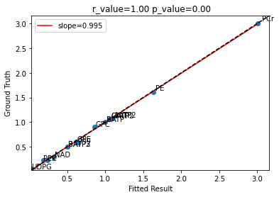
[31]:
(0.9954449822381952, 0.9992212974530363, 4.645693969839231e-21)
[ ]: