Speed Up Batch Fitting Using Multiprocessing
Example: Dynamic Unlocalized Phosphorus MRS
2024-01-30 CSI AMARES Fitting (IOWA)/Data/Phosphorus/Acceptable_quality_tibialisThis tutorial demonstrates how to use the pyAMARES library to analyze 31P MRS data.
Data provided by michael.vaeggemose@gehealthcare.com.
Files:
Prior Knowledge File (CSV Format)
Filename:
JJM_3T_v3.csvDescription: Converted from the OXSA prior knowledge file
AMARES.priorKnowledge.PK_31P_3T_muscle_AS_TA_171122_JJM.m.
P-File (Matlab Format)
Filename:
20230922_091144_P51200.matDescription: Raw data file from MRI in Matlab format for processing.
PyAMARES can be installed by !pip install pyAMARES in the Jupyter notebook cell, or pip install pyAMARES in the terminal.
Import needed libraries, including pyAMARES
[1]:
import numpy as np
import matplotlib.pyplot as plt
from scipy import io
import pyAMARES

pyAMARES.__version__
[1]:
'0.3.15'
Load Matlab file into python using scipy.io.loadmat or mat73.loadmat
[2]:
filename = "20230922_091144_P51200.matlabfile.mat"
matdic = io.loadmat(filename)
matdic.keys()
[2]:
dict_keys(['__header__', '__version__', '__globals__', 'h', 'spec', 'par', 'fid', 'hz'])
Extract header parameters and data used for AMARES fitting
[3]:
h = matdic["h"]
par = matdic["par"]
spec = matdic["spec"]
fidarr = matdic["fid"]
fidarr.shape
[3]:
(375, 1024)
[4]:
TR = h["image"][0, 0]["tr"][0, 0][0, 0] * 1e-6
f0_avg = float(par["f0"][0][0][0][0])
sw = float(par["bw"][0][0][0][0])
samples = float(par["samples"][0][0][0][0])
dwellTime = 1 / sw
fact = 2
beginTime = fact * h["rdb_hdr"][0, 0]["te"][0, 0][0, 0] / 2 * 1e-6
bofreq = f0_avg / 1e6  # convert to MHz
Remove dummy scans – approx 10 points
[5]:
fid = fidarr[9:, :]
time_axis = np.linspace(0, fid.shape[0] * TR, fid.shape[0])
[6]:
beginTime, fid.shape, len(time_axis)
[6]:
(0.000455, (366, 1024), 366)
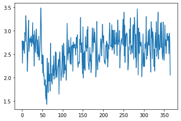
Check the SNR of the input FIDs
[7]:
snrlist = []
for i in range(fid.shape[0]):
    snrlist.append(
        pyAMARES.kernel.fid.fidSNR(fid[i, :], indsignal=(0, 10), pts_noise=50)
    )
snrlist = np.array(snrlist)
plt.plot(snrlist)
[7]:
[<matplotlib.lines.Line2D at 0x7fc2488a0580>]
Start AMARES fitting
Initialize FID Data and Fitting Parameter Object using pyAMARES.initialize_FID
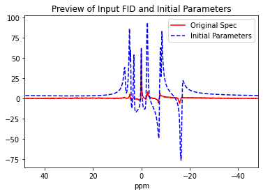
- Initialize Fitting ParametersBegin by setting up the initial fitting parameters.
- Preview the Loaded ParametersDisplay the parameters in a figure to visually verify and adjust as needed.
- Preview the Loaded Prior Knowledge TableDisplay the prior knowledge table, which has been converted from the MATLAB file
AMARES.priorKnowledge.PK_31P_3T_muscle_AS_TA_171122_JJM.m, to ensure it faithfully reproduces the OXSA’s prior knowledge dataset.
[8]:
# Normalize and calculate the mean FID from all FIDs
fid2 = fid / np.max(np.abs(fid))
fidsum = np.mean(fid2, axis=0)
[9]:
pkfile = "JJM_3T_v3.csv"
FIDobj = pyAMARES.initialize_FID(
    fidsum,
    priorknowledgefile=pkfile,
    MHz=bofreq,
    sw=sw,
    deadtime=beginTime,
    normalize_fid=False,
    flip_axis=False,
    preview=True,
)
Checking comment lines in the prior knowledge file
Printing the Prior Knowledge File JJM_3T_v3.csv
| PCr | PME | Pia | Pib | PDE | BATP | BATP2 | BATP3 | AATP | AATP2 | GATP | GATP2 | NAD | |
|---|---|---|---|---|---|---|---|---|---|---|---|---|---|
| Index | |||||||||||||
| Initial Values | NaN | NaN | NaN | NaN | NaN | NaN | NaN | NaN | NaN | NaN | NaN | NaN | NaN |
| amplitude | 1 | 1 | 1 | 1 | 1 | 1 | BATP/2 | BATP/2 | 1 | AATP | 1 | GATP | 1 |
| chemicalshift | 0 | 6.7 | 4.83 | 4.38 | 3.02 | -16.54 | BATP-15Hz | BATP+15Hz | -7.48 | AATP-16Hz | -2.22 | GATP-15Hz | -8.4 |
| linewidth | 20 | 40 | 20 | 20 | 20 | 20 | BATP | BATP | 20 | AATP | 20 | GATP | 20 |
| phase | 0 | PCr | PCr | PCr | PCr | PCr | PCr | PCr | PCr | PCr | PCr | PCr | PCr |
| g | 0 | 0 | 0 | 0 | 0 | 0 | 0 | 0 | 0 | 0 | 0 | 0 | 0 |
| Bounds | NaN | NaN | NaN | NaN | NaN | NaN | NaN | NaN | NaN | NaN | NaN | NaN | NaN |
| amplitude | (0, | (0, | (0, | (0, | (0, | (0, | (0, | (0, | (0, | (0, | (0, | (0, | (0, |
| chemicalshift | (-0.5,0.2) | (6.00, 7.10) | (4.19,5.03) | (3.69, 4.39) | (2.87, 3.27) | (-17,-15) | (-17,-15) | (-17,-15) | (-8,-6) | (-8,-6) | (-3,-2) | (-3,-2) | (-8.45, -8.35) |
| linewidth | (3,23) | (10,60) | (5,30) | (5,30) | (5,50) | (0, | (0, | (0, | (0, | (0, | (0, | (0, | (5,30) |
| phase | (-180, 180) | (-180, 180) | (-180, 180) | (-180, 180) | (-180, 180) | (-180, 180) | (-180, 180) | (-180, 180) | (-180, 180) | (-180, 180) | (-180, 180) | (-180, 180) | (-180, 180) |
| g | (0,1) | (0,1) | (0,1) | (0,1) | (0,1) | (0,1) | (0,1) | (0,1) | (0,1) | (0,1) | (0,1) | (0,1) | (0,1) |
| NaN | NaN | NaN | NaN | NaN | NaN | NaN | NaN | NaN | NaN | NaN | NaN | NaN | NaN |
Initialize Fitting Parameters from the Mean Spectrum
Fitting Strategies There are two primary fitting methods available:
leastsq: Levenberg-Marquardt Algorithm
Speed: Faster
Description: Levenberg-Marquardt algorithm, can be used to obtain the initial fitting parameters for
least_squares.
least_squares: Trust Region Reflective Method
Speed: Slower
Description: Trust Region Reflective, the method used in OXSA. Though it is slower, it often yields better fitting results.
[10]:
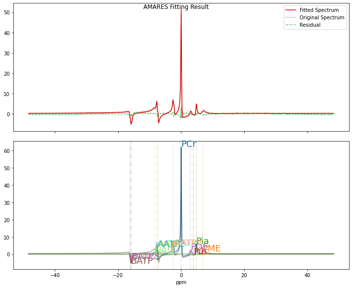
out1 = pyAMARES.fitAMARES(
    fid_parameters=FIDobj,
    fitting_parameters=FIDobj.initialParams,
    method="leastsq",
    ifplot=True,
    inplace=False,
)
A copy of the input fid_parameters will be returned because inplace=False
Autogenerated tol is 7.949e-07
Fitting with method=leastsq took 4.872845 seconds
Estimated CRLBs are calculated using the default noise variance estimation used by OXSA.
/home/jxu125/git/pyamares/pyAMARES/util/crlb.py:54: RuntimeWarning: Warning: The matrix may be ill-conditioned. Condition number is high: 1.441e+14
  warnings.warn(
a_sd is all None, use crlb instead!
freq_sd is all None, use crlb instead!
lw_sd is all None, use crlb instead!
phase_sd is all None, use crlb instead!
g_std is all None, use crlb instead!
Lmfit Fitting Results:
----------------
Number of function evaluations (nfev): 1000
Reduced chi-squared (redchi): 0.00022850571236512654
Fit success status: Failure
Fit message: Tolerance seems to be too small. Could not estimate error-bars.
Norm of residual = 0.462
Norm of the data = 11.827
resNormSq / dataNormSq = 0.039
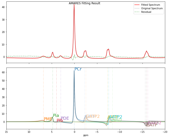
Modify the plotting parameters to visualize the AMARES fitting results.
[11]:
plotParameters = (
    FIDobj.plotParameters
)  # Get the template of plotParameters from an FID object
plotParameters.xlim = (15, -20)  # Set the ppm range from 15 to -20 ppm
plotParameters.ifphase = True  # Enable phasing of the spectrum for better visualization. Note: As AMARES utilizes a time-domain fitting strategy,
# phasing the FID is not required for the fitting process but may be useful for visualization.
plotParameters.lb = 5.0  # linebroadening of 5 Hz
plotParameters
[11]:
Namespace(deadtime=0.000455, ifphase=True, lb=5.0, sw=5000.0, xlim=(15, -20))
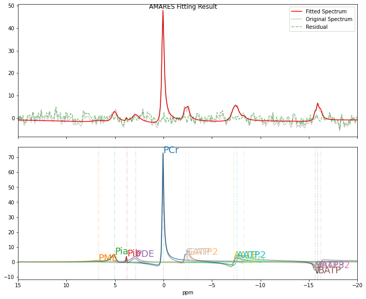
Visualization of the AMARES Fitting Result (Optional)
This section demonstrates how to plot the fitting results using the
pyAMARES.plotAMARESfunction.
[12]:
pyAMARES.plotAMARES(
    fid_parameters=out1,  # `out1` is the output from `fitAMARES` containing the fitted parameters.
    fitted_params=out1.fittedParams,  # # Optional: If omitted, `out1.fittedParams` is used by default.
    plotParameters=plotParameters,
)
The fitted parameters of the mean spectrum can be accessed using out1.fittedParams.
[13]:
out1.fittedParams
[13]:
| name | value | initial value | min | max | vary | expression |
|---|---|---|---|---|---|---|
| ak_PCr | 0.42801070 | 1.0 | 0.00000000 | inf | True | |
| freq_PCr | 0.99136334 | 0.0 | -25.8603225 | 10.3441290 | True | |
| dk_PCr | 33.1927771 | 62.83185307179586 | 0.00000000 | 72.2566310 | True | |
| phi_PCr | -0.30070732 | 0.0 | -3.14159265 | 3.14159265 | True | |
| g_PCr | 0.00000000 | 0.0 | 0.00000000 | 1.00000000 | False | |
| ak_PME | 0.08179148 | 1.0 | 0.00000000 | inf | True | |
| freq_PME | 352.457521 | 346.5283215 | 310.323870 | 367.216579 | True | |
| dk_PME | 188.495559 | 125.66370614359172 | 0.00000000 | 188.495559 | True | |
| phi_PME | -0.30070732 | 0.0 | -3.14159265 | 3.14159265 | False | phi_PCr |
| g_PME | 0.00000000 | 0.0 | 0.00000000 | 1.00000000 | False | |
| ak_Pia | 0.07026761 | 1.0 | 0.00000000 | inf | True | |
| freq_Pia | 246.430174 | 249.81071534999998 | 216.709503 | 260.154844 | True | |
| dk_Pia | 53.8685244 | 62.83185307179586 | 0.00000000 | 94.2477796 | True | |
| phi_Pia | -0.30070732 | 0.0 | -3.14159265 | 3.14159265 | False | phi_PCr |
| g_Pia | 0.00000000 | 0.0 | 0.00000000 | 1.00000000 | False | |
| ak_Pib | 1.6481e-06 | 1.0 | 0.00000000 | inf | True | |
| freq_Pib | 204.144163 | 226.53642509999997 | 190.849180 | 227.053632 | True | |
| dk_Pib | 5.94144907 | 62.83185307179586 | 0.00000000 | 94.2477796 | True | |
| phi_Pib | -0.30070732 | 0.0 | -3.14159265 | 3.14159265 | False | phi_PCr |
| g_Pib | 0.00000000 | 0.0 | 0.00000000 | 1.00000000 | False | |
| ak_PDE | 0.05883560 | 1.0 | 0.00000000 | inf | True | |
| freq_PDE | 155.759171 | 156.1963479 | 148.438251 | 169.126509 | True | |
| dk_PDE | 108.069092 | 62.83185307179586 | 0.00000000 | 157.079633 | True | |
| phi_PDE | -0.30070732 | 0.0 | -3.14159265 | 3.14159265 | False | phi_PCr |
| g_PDE | 0.00000000 | 0.0 | 0.00000000 | 1.00000000 | False | |
| ak_BATP | 0.05341679 | 1.0 | 0.00000000 | inf | True | |
| freq_BATP | -824.492774 | -855.4594682999999 | -879.250965 | -775.809675 | True | |
| dk_BATP | 42.8820085 | 62.83185307179586 | 0.00000000 | inf | True | |
| phi_BATP | -0.30070732 | 0.0 | -3.14159265 | 3.14159265 | False | phi_PCr |
| g_BATP | 0.00000000 | 0.0 | 0.00000000 | 1.00000000 | False | |
| ak_BATP2 | 0.02670840 | 0.5 | 0.00000000 | inf | False | ak_BATP/2 |
| freq_BATP2 | -839.492774 | -870.4594682999999 | -879.250965 | -775.809675 | False | freq_BATP-15 |
| dk_BATP2 | 42.8820085 | 62.83185307179586 | 0.00000000 | inf | False | dk_BATP |
| phi_BATP2 | -0.30070732 | 0.0 | -3.14159265 | 3.14159265 | False | phi_PCr |
| g_BATP2 | 0.00000000 | 0.0 | 0.00000000 | 1.00000000 | False | |
| ak_BATP3 | 0.02670840 | 0.5 | 0.00000000 | inf | False | ak_BATP/2 |
| freq_BATP3 | -809.492774 | -840.4594682999999 | -879.250965 | -775.809675 | False | freq_BATP+15 |
| dk_BATP3 | 42.8820085 | 62.83185307179586 | 0.00000000 | inf | False | dk_BATP |
| phi_BATP3 | -0.30070732 | 0.0 | -3.14159265 | 3.14159265 | False | phi_PCr |
| g_BATP3 | 0.00000000 | 0.0 | 0.00000000 | 1.00000000 | False | |
| ak_AATP | 0.06773969 | 1.0 | 0.00000000 | inf | True | |
| freq_AATP | -377.396563 | -386.8704246 | -413.765160 | -310.323870 | True | |
| dk_AATP | 41.7646910 | 62.83185307179586 | 0.00000000 | inf | True | |
| phi_AATP | -0.30070732 | 0.0 | -3.14159265 | 3.14159265 | False | phi_PCr |
| g_AATP | 0.00000000 | 0.0 | 0.00000000 | 1.00000000 | False | |
| ak_AATP2 | 0.06773969 | 1.0 | 0.00000000 | inf | False | ak_AATP |
| freq_AATP2 | -393.396563 | -402.8704246 | -413.765160 | -310.323870 | False | freq_AATP-16 |
| dk_AATP2 | 41.7646910 | 62.83185307179586 | 0.00000000 | inf | False | dk_AATP |
| phi_AATP2 | -0.30070732 | 0.0 | -3.14159265 | 3.14159265 | False | phi_PCr |
| g_AATP2 | 0.00000000 | 0.0 | 0.00000000 | 1.00000000 | False | |
| ak_GATP | 0.05759985 | 1.0 | 0.00000000 | inf | True | |
| freq_GATP | -117.113245 | -114.81983190000001 | -155.161935 | -103.441290 | True | |
| dk_GATP | 48.9614629 | 62.83185307179586 | 0.00000000 | inf | True | |
| phi_GATP | -0.30070732 | 0.0 | -3.14159265 | 3.14159265 | False | phi_PCr |
| g_GATP | 0.00000000 | 0.0 | 0.00000000 | 1.00000000 | False | |
| ak_GATP2 | 0.05759985 | 1.0 | 0.00000000 | inf | False | ak_GATP |
| freq_GATP2 | -132.113245 | -129.8198319 | -155.161935 | -103.441290 | False | freq_GATP-15 |
| dk_GATP2 | 48.9614629 | 62.83185307179586 | 0.00000000 | inf | False | dk_GATP |
| phi_GATP2 | -0.30070732 | 0.0 | -3.14159265 | 3.14159265 | False | phi_PCr |
| g_GATP2 | 0.00000000 | 0.0 | 0.00000000 | 1.00000000 | False | |
| ak_NAD | 0.02618298 | 1.0 | 0.00000000 | inf | True | |
| freq_NAD | -434.453418 | -434.453418 | -437.039450 | -431.867386 | True | |
| dk_NAD | 92.0581523 | 62.83185307179586 | 0.00000000 | 94.2477796 | True | |
| phi_NAD | -0.30070732 | 0.0 | -3.14159265 | 3.14159265 | False | phi_PCr |
| g_NAD | 0.00000000 | 0.0 | 0.00000000 | 1.00000000 | False |
Accessing Detailed Fitting Results in the FID object, such as out1
Detailed Peak Parameters including Multiplets
Variable:
out1.result_multipletDescription: Contains the fitted parameters for each peak, including sub-peaks within multiplets.
Peak Parameters
Variable:
out1.result_sumDescription: Provides the summation of all multiplets, offering a consolidated view of the spectrum’s fitting results.
Enhanced Visualization of Data
Variable:
out1.styled_dfDescription: This data frame is styled to highlight statistical reliability, color-coding entries where the Cramer-Rao Lower Bounds (CRLB) are less than 20%. This visualization aids in identifying the most statistically reliable parameters.
[14]:
out1.styled_df
[14]:
| amplitude | sd | CRLB(%) | chem shift(ppm) | sd(ppm) | CRLB(cs%) | LW(Hz) | sd(Hz) | CRLB(LW%) | phase(deg) | sd(deg) | CRLB(phase%) | g | g_sd | g (%) | SNR | |
|---|---|---|---|---|---|---|---|---|---|---|---|---|---|---|---|---|
| name | ||||||||||||||||
| PCr | 0.428 | 0.003 | 0.622 | 0.019 | 0.001 | 4.676 | 10.566 | 0.091 | 0.864 | -17.229 | -0.368 | 2.136 | 0.000 | nan | nan | 49.769 |
| PME | 0.082 | 0.007 | 9.106 | 6.815 | 0.044 | 0.644 | 60.000 | 7.111 | 11.851 | -17.229 | -0.368 | 2.136 | 0.000 | nan | nan | 9.511 |
| Pia | 0.070 | 0.004 | 5.146 | 4.765 | 0.008 | 0.164 | 17.147 | 1.198 | 6.984 | -17.229 | -0.368 | 2.136 | 0.000 | nan | nan | 8.171 |
| Pib | 0.000 | 0.001 | 81244.631 | 3.947 | 18.202 | 461.156 | 1.891 | 3084.591 | 163100.438 | -17.229 | -0.368 | 2.136 | 0.000 | nan | nan | 0.000 |
| PDE | 0.059 | 0.005 | 9.009 | 3.012 | 0.026 | 0.877 | 34.399 | 4.172 | 12.127 | -17.229 | -0.368 | 2.136 | 0.000 | nan | nan | 6.841 |
| BATP | 0.107 | 0.003 | 3.269 | -15.941 | -0.007 | 0.046 | 13.650 | 0.976 | 7.151 | -17.229 | -0.368 | 2.136 | 0.000 | nan | nan | 12.423 |
| AATP | 0.135 | 0.004 | 2.775 | -7.297 | -0.005 | 0.063 | 13.294 | 0.637 | 4.795 | -17.229 | -0.368 | 2.136 | 0.000 | nan | nan | 15.754 |
| GATP | 0.115 | 0.004 | 3.233 | -2.264 | -0.007 | 0.299 | 15.585 | 0.969 | 6.219 | -17.229 | -0.368 | 2.136 | 0.000 | nan | nan | 13.395 |
| NAD | 0.026 | 0.005 | 20.577 | -8.400 | -0.048 | 0.570 | 29.303 | 7.850 | 26.789 | -17.229 | -0.368 | 2.136 | 0.000 | nan | nan | 3.045 |
DC correction
[15]:
quarter_length = round(FIDobj.timeaxis.shape[0] * 0.25)  # 1/4, 256 points
fid3 = np.zeros(fid2.shape, dtype=fid2.dtype)
dc_offset_arr = np.mean(fid2[:, -quarter_length - 1 :], axis=1)
fid3 = fid2 - dc_offset_arr[:, np.newaxis]
print("DC correction by the mean of the last %i points" % quarter_length)
DC correction by the mean of the last 256 points
Futher Optimization of Initial Parameters for batch fitting (Optional)
[16]:
FIDobj.fid = fid3[
    1, :
]  # Update the FID in the FIDobj to the first spectrum of DC-corrected FIDs.
out2 = pyAMARES.fitAMARES(
    fid_parameters=FIDobj,
    fitting_parameters=out1.fittedParams,  # You can use either FIDobj.initialParameters, which are directly loaded from the prior knowledge,
    # or the fitted parameters from a previous round of AMARES fitting, such as out1.fittedParams.
    method="least_squares",
    ifplot=True,
    inplace=False,
)
A copy of the input fid_parameters will be returned because inplace=False
Autogenerated tol is 9.188e-07
Fitting with method=least_squares took 3.171307 seconds
Estimated CRLBs are calculated using the default noise variance estimation used by OXSA.
Lmfit Fitting Results:
----------------
Number of function evaluations (nfev): 15
Reduced chi-squared (redchi): 0.01191279256392595
Fit success status: Success
Fit message: `ftol` termination condition is satisfied.
Norm of residual = 24.064
Norm of the data = 38.047
resNormSq / dataNormSq = 0.632
Fitted Results from the First FID:
The results obtained from fitting a single FID are less reliable than those derived from the mean spectrum.
[17]:
out2.styled_df
[17]:
| amplitude | sd | CRLB(%) | chem shift(ppm) | sd(ppm) | CRLB(cs%) | LW(Hz) | sd(Hz) | CRLB(LW%) | phase(deg) | sd(deg) | CRLB(phase%) | g | g_sd | g (%) | SNR | |
|---|---|---|---|---|---|---|---|---|---|---|---|---|---|---|---|---|
| name | ||||||||||||||||
| PCr | 0.452 | 0.017 | 3.717 | 0.026 | 0.005 | 18.350 | 9.374 | 0.499 | 5.178 | -19.355 | 2.269 | 11.413 | 0.000 | 0.000 | nan | 2.683 |
| PME | 0.031 | 0.057 | 180.420 | 6.697 | 0.837 | 12.167 | 60.000 | 141.056 | 228.880 | -19.355 | 2.269 | 11.413 | 0.000 | 0.000 | nan | 0.181 |
| Pia | 0.094 | 0.036 | 36.839 | 5.030 | 0.079 | 1.530 | 26.746 | 12.936 | 47.089 | -19.355 | 2.269 | 11.413 | 0.000 | 0.000 | nan | 0.560 |
| Pib | 0.006 | 0.009 | 149.109 | 3.762 | 0.027 | 0.706 | 1.167 | 4.995 | 416.694 | -19.355 | 2.269 | 11.413 | 0.000 | 0.000 | nan | 0.033 |
| PDE | 0.107 | 0.044 | 40.011 | 2.870 | 0.149 | 5.038 | 44.319 | 24.075 | 52.886 | -19.355 | 2.269 | 11.413 | 0.000 | 0.000 | nan | 0.633 |
| BATP | 0.130 | 0.022 | 16.157 | -15.933 | 0.029 | 0.179 | 11.094 | 3.659 | 32.110 | -19.355 | 2.269 | 11.413 | 0.000 | 0.000 | nan | 0.771 |
| AATP | 0.184 | 0.042 | 22.216 | -7.262 | 0.066 | 0.887 | 28.950 | 11.450 | 38.504 | -19.355 | 2.269 | 11.413 | 0.000 | 0.000 | nan | 1.090 |
| GATP | 0.110 | 0.024 | 21.246 | -2.254 | 0.042 | 1.835 | 14.252 | 5.920 | 40.442 | -19.355 | 2.269 | 11.413 | 0.000 | 0.000 | nan | 0.655 |
| NAD | 0.011 | 0.023 | 205.125 | -8.350 | 0.197 | 2.291 | 11.838 | 31.881 | 262.197 | -19.355 | 2.269 | 11.413 | 0.000 | 0.000 | nan | 0.066 |
Batch Fitting: Loop to get all amplitude results
run_parallel_fitting_with_progressis designed to batch fit multiple FIDs simultaneously, utilizing a specified number of CPUs to enhance speed performance.It typically takes 7~10 min to fit 366 FIDs using the 2 CPUs available of Google Colab.
[18]:
fid3.shape
[18]:
(366, 1024)
[19]:
result_list = pyAMARES.run_parallel_fitting_with_progress(
    fid3,  # 2D array of FIDs. Here, `fid3.shape=(366,1024)` indicates 366 FIDs, each with 1024 points.
    FIDobj_shared=out2,  # Use the FID object `out2` for fitting all FIDs.
    initial_params=out2.fittedParams,  # Use the fitted results of the first FID as the initial parameters.
    num_workers=30,  # Parallel processing with 2 sessions if used in Google Colab, suitable for the 2 CPUs available in Google Colab.
    initialize_with_lm=True,
    method="leastsq",
)  # Use the Levenberg-Marquardt method by default for faster processing.
Fitting 366 spectra with 30 processors took 101 seconds
Smoothing data
[20]:
amplist = []
for out_table in result_list:
    amplist.append(out_table["amplitude"].values)
fid_amp = np.array(amplist)
fid_amp.shape
[20]:
(366, 13)
Define a smooth function to mimic smooth in Matlab
[21]:
def smooth(x, window_len=11, window="hanning", verbose=False):
    if x.ndim != 1:
        raise ValueError("smooth only accepts 1 dimension arrays.")

    if x.size < window_len:
        raise ValueError("Input vector needs to be bigger than window size.")

    if window_len < 3:
        return x

    if window not in ["flat", "hanning", "hamming", "bartlett", "blackman"]:
        raise ValueError(
            "Window is on of 'flat', 'hanning', 'hamming', 'bartlett', 'blackman'"
        )

    s = np.r_[x[window_len - 1 : 0 : -1], x, x[-2 : -window_len - 1 : -1]]
    if window == "flat":  # moving average
        w = np.ones(window_len, "d")
    else:
        w = eval("np." + window + "(window_len)")

    y = np.convolve(w / w.sum(), s, mode="valid")
    if verbose:
        print("input len", len(x))
        print("output len", len(y))
    y2 = y[(window_len // 2) : -(window_len // 2)]
    if verbose:
        print("output len", len(y2))
    return y2
Determine PCr rise time
[22]:
fid_amp.shape[0]
kinec_smooth = 11
fid_amp_smooth = np.zeros_like(
    fid_amp
)  # Initialize fid_amp_smooth with the same shape and type as fid_amp
for i in range(fid_amp.shape[1]):
    fid_amp_smooth[:, i] = smooth(fid_amp[:, i], kinec_smooth, verbose=False)
[23]:
recovery_start_time = np.argmin(fid_amp_smooth[:, 0])
recovery_end_time = fid_amp_smooth.shape[0]  # or simply len(fid_amp_smooth)

PCr_recovery_raw = fid_amp[recovery_start_time:recovery_end_time, 0]  # Raw PCr data
PCr_recovery_avg = fid_amp_smooth[
    recovery_start_time:recovery_end_time, 0
]  # Smoothed PCr data
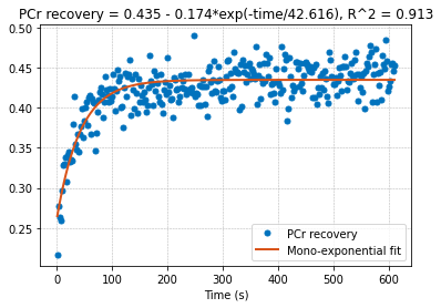
[24]:
from scipy.optimize import curve_fit


t_rec = TR * (np.arange(len(PCr_recovery_avg)) + 1)


# Define the mono-exponential function to fit
def mono_exp(x, a, b, c):
    return a - b * np.exp(-x / c)


# Initial guess for the parameters
initial_guess = [
    np.max(PCr_recovery_avg),
    np.max(PCr_recovery_avg) - np.min(PCr_recovery_avg),
    1,
]

# Perform the fit
params, cov = curve_fit(mono_exp, t_rec, PCr_recovery_avg, p0=initial_guess)

# Use the fitted parameters to generate the fitted curve
xx = np.linspace(1, TR * len(PCr_recovery_avg), len(PCr_recovery_avg))
fitted_curve = mono_exp(xx, *params)
[25]:
# Use the fitted parameters to calculate the predicted values
predicted = mono_exp(t_rec, *params)

# Calculate the total sum of squares (SST)
sst = np.sum((PCr_recovery_avg - np.mean(PCr_recovery_avg)) ** 2)

# Calculate the residual sum of squares (SSR)
ssr = np.sum((PCr_recovery_avg - predicted) ** 2)

# Calculate R^2
r_squared = 1 - (ssr / sst)

print("R^2:", r_squared)
R^2: 0.913155558241575
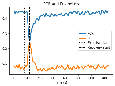
Plot data
[26]:
plt.figure()
plt.plot(time_axis, fid_amp_smooth[:, 0], linewidth=3, label="PCR")
plt.plot(
    time_axis, fid_amp_smooth[:, 2] + fid_amp_smooth[:, 3], linewidth=3, label="Pi"
)
plt.title("PCR and Pi kinetics")
plt.xlabel("Time (s)")
plt.legend(loc=3)

# Adding vertical lines for exercise start and recovery start
plt.axvline(x=80, linestyle=":", color="k", linewidth=2, label="Exercise start")
plt.axvline(
    x=time_axis[recovery_start_time],
    linestyle="--",
    color="k",
    linewidth=2,
    label="Recovery start",
)

plt.legend()
plt.show()
[27]:
plt.figure()
plt.plot(
    xx,
    PCr_recovery_raw,
    ".",
    color=[0, 0.4470, 0.7410],
    markersize=10,
    label="PCr recovery",
)
plt.plot(
    xx,
    fitted_curve,
    "-",
    color=[0.8500, 0.3250, 0.0980],
    linewidth=2,
    label="Mono-exponential fit",
)

# Assuming f0_avg has attributes 'a', 'b', 'c' for the fit parameters and gof_avg has an attribute 'rsquare' for R^2
plt.title(
    f"PCr recovery = {round(params[0], 3)} - {round(params[1], 3)}*exp(-time/{round(params[2], 3)}), R^2 = {round(r_squared, 3)}"
)
plt.xlabel("Time (s)")
plt.grid(True, which="both", linestyle="--", linewidth=0.5)
plt.legend(loc=4)
plt.show()
[ ]: